Large-Scale HTS Reconciliation

Reconciling large-scale time-series forecasts on systems with tight memory limit and non-uniform data access latency.

GitHub Repository

Summary

We present the design and implementation of a system that performs forecast reconciliation for large-scale, hierarchical time-series datasets. The system features various forms of parallelization (shared-memory, message-passing, SIMD) of multiple reconciliation methods (top-down, bottom-up, middle-out, OLS, and WLS) on single-node, multi-core, and multi-node CPU platforms using Eigen, OpenMP, and OpenMPI. It is suitable for heavy workloads on platforms with non-uniform data access latency for individual forecasts, where communication- and computation-reduction techniques have demonstrated up to 1000x speed-up compared to existing open-source alternatives (Nixtla HierarchicalForecast v0.2.1) utilizing dense matrix multiplication. In addition, we have also created three large-scale time-series forecasting benchmarks (M5-Hobbies, M5-Full and Wikipedia), which contain hierarchical information that are orders of magnitude richer than existing academic counterparts. The resulting artifact is a Python package, LHTS, that invokes optimized reconciliation routines written in C++ on numeric NumPy matrices in single- and multi-process settings. A demo of integration of our package into a regular multi-process time-series forecasting workload involving a popular forecasting system, Prophet, is also provided and studied.

Background

The Problem

Time-series forecasting is a very popular field in statistical and machine learning and has many applications in financial markets (predicting stocks), IoT (predicting sensors), geosciences (predicting earthquakes), etc. Time-series is usually represented as a list of values y₁⋯y_k with timestamps t₁⋯t_k associated with each value, and the task of forecasting could be defined as "extending" the values to certain time stamps t_k + 1⋯t_k + l into the future y_k + 1⋯y_k + l [Hyndman and Athanasopoulos, 2021].

Oftentimes, the time-series in a forecasting workload can be organized by certain characteristics of interest, which can naturally be aggregated into different levels of a hierarchy. For example, if one were to forecast Australia's domestic visitors per day [Panagiotelis et al., 2021], one would be additionally interested in city-level, state-level, or nation-level forecasts. Notably, these forecasts have constraints placed on some of them with respect to the hierarchy; e.g., a state's forecast is the sum of all of the cities' forecasts. Thus, a natural question arises:

How can we effectively leverage the structural information in the hierarchy to make forecasts on all levels more accurate in a more efficient manner?

The Algorithm

In most settings, the algorithm forecasting individual time-series is oblivious of the above-mentioned hierarchy, hence the manuscript focuses on a reconciliation-oriented approach, where forecasts are individually produced for each entity Ŷ_v (for node v in the directed graph of hierarchy G = {V, E}), and the goal would be to find a way to "reconcile" each forecast to produce $\overline{Y}_v$ such that they conform to the constraints imposed by the hierarchy (such as parent equalling to sum of children) and more desirably, achieves a better performance metric ℒ across all levels $\Sigma_{v \in V}\mathcal{L}(Y_v, \overline{Y}_v)$. The set of updated forecasts $\overline{Y}_v$ is often called coherent forecasts. This approach is intuitive because e.g. 1: if the model independently predicts tourism on city level and on state level, it is very unlikely that the city-level forecast could sum to that of the state-level naively; 2: there are patterns within the state-level forecast than can help improve city-level forecast, and vice versa.

Not all nodes v are required to be forecasted for a successful reconciliation. Here presents five popular methods, each of which has different requirements on nodes to forecast to produce a coherent forecast:

1. Bottom-up [Hyndman and Athanasopoulos, 2021]: produce forecast for all leaves, then gradually aggregating up to root (via summing or other methods).

2. Top-down [Hyndman and Athanasopoulos, 2021]: produce forecast for root only, then specify, at each level, how a parent forecast breaks down to its children. Then execute the gradual breakdown as we go down the levels.

3. Middle-out [Hyndman and Athanasopoulos, 2021]: pick a level that is not the leaves nor the root, generate forecasts, then produce bottom-up for all levels above and top-down for all levels below.

4. OLS [Hyndman et al., 2011] (Ordinary Least Square): produce forecast for all nodes, then multiply by reconciliation matrix G = (S^TS)^− 1S^T, where S is the summing matrix (explained below).

5. WLS [Athanasopoulos et al., 2017] (Weighted Least Square): produce forecast for all nodes, then multiply by reconciliation matrix G = (S^TWS)^− 1S^TW for some diagonal matrix W, where S is the summing matrix (explained below).

Before discussing the parallelization of forecast reconciliation, it's useful to remark that forecasts on each node are independent, and therefore are naively parallelizable. Thus, a usage pattern we often observe in production is each core c_i producing a subset of forecast:

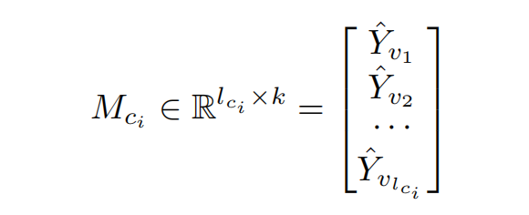
represented as a matrix of dimension (number of forecasts the core is responsible for) times (time horizon). The matrices of each node will reside on memory close to the core in a NUMA (non-uniform memory access) architecture, and, with individual forecasts within a hierarchy scattered across many cores, time for a particular process to access a particular node's forecast is also highly non-uniform with respect to the interconnect topology. As discussed in the following section, this setting has profound implications in terms of performance of reconciliation algorithms on parallel machines. For now, the assumption is that the matrices on each process is collected and vertically stacked into a single matrix representing all forecasts, as shown in the right hand side of Figure 1 below.

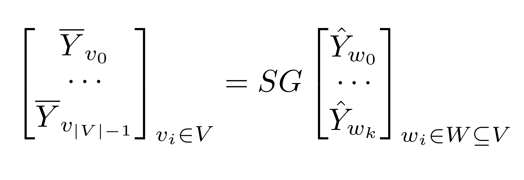
In addition to naively reconciling forecast node-by-node along the graph hierarchy in a sequential way, there are a few works on a single-process parallelization technique inspired by matrix algebra. The core intuition of the existing approach is that if repetitive computations are allowed, aggregation of each node in the hierarchy can be thought of as independent computations [Hyndman et al., 2011]. This allows an elegant matrix-multiplication-based interpretation of the reconciliation problem, reformulated as a multiplication by G (the reconciliation matrix) to map partial forecasts from nodes W to base level forecasts, then summing up to each node via S (the summing matrix) to obtain the full forecast of nodes in V:

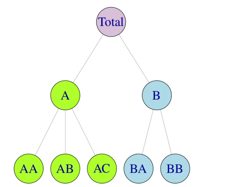
This can be seen as the "pseudo-code" of the baseline algorithm. For example, given the following hierarchy in Figure 1 in [Hyndman and Athanasopoulos, 2021], a bottom-up approach would have a reconciliation matrix

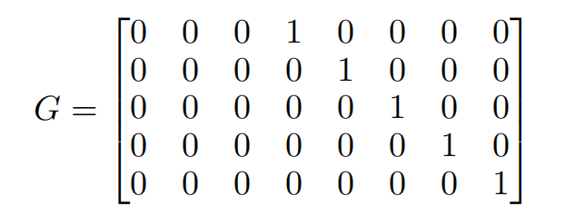
and a summing matrix S bearing a relationship like

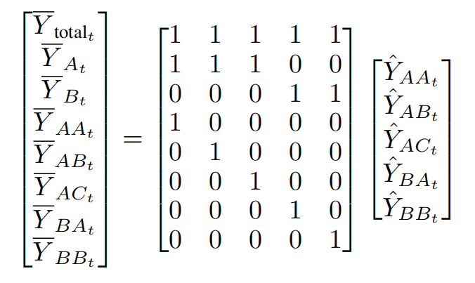
The computational intensity matrix multiplication paves the way for speed-up using optimized libraries like BLAS (Basic Linear Algebra Subprograms, [Lawson et al., 1979]), leveraging SIMD and threaded-parallelism. Commercial, open-sourced solutions like Nixtla HierarchicalForecast [Olivares et al., 2022] also utilize this property.

The Challenge

On the first look, the matrix-based solution in a single process seems to be efficient enough and embarrassingly parallel. Below illustrates why this notion is wrong, espcially when the workload is scaling with memory constraints and the forecasts start off in different memory locations with non-uniform access cost.

The Constraints

Real-world hierarchical time-series forecast datasets are large and unsuitable for the naive dense-matrix-based parallelization technique. For example, the Web Traffic Time Series Forecasting [Kaggle, b] contains 145,063 time-series for 551 time-stamps across multiple hierarchies (e.g. locale, access, agent), which places a lower bound of 145063² × 4 ≈ 84.17 gigabytes to store the summing and reconciliation matrices in dense format, not to mention the time it takes to perform the matrix multiplication. The difficulty therefore lies in how to efficiently design an algorithm that has less memory footprint while efficiently parallelizing the reconciliation.

Furthermore, matrix multiplication in a reconciliation workload are sparse in nature. The summing matrix S, from how it's defined, only contains up to O(nlogn) non-zero entries among O(n²) total entries, and the reconciliation matrix G are also very sparse for bottom-up, top-down and middle-out methods. The result is wasted computation on zero-entries in dense-dense matrix multiplications of SG and SGY.

Finally, under a multiprocess setting, the forecasts before reconciliation are spread across many processes on cores that are far away from each other. Devising an efficient method to distribute the computation across different processes while minimizing communication is equally challenging.

The Workload

Data dependencies and memory access characteristics of the forecast reconciliation workload tie back to the graph structure of the hierarchy. All processes require a copy of the hierarchy itself to be aware of where communication takes place. Based on communication and computation intensity, we need to also devise non-trivial strategies for splitting up work into chunks owned by each process, even when assuming that producing the forecast for each is uniform. For bottom-up, top-down and middle-out approaches respectively, node that are closer to the leaves/root/selected level require less work to produce than others. The different choices may result in divergent execution or workload imbalance. Locality also exists in this place based on where forecasts are originally: processes only need to communicate with each other forecasts that are necessary for aggregation (instead of all); if all forecasts of a certain level exists on a process in the first place, we could eliminate communication altogether in the round. This intricate interplay between graph topology and communication-to-computation ratio also presents a challenge in optimizing our system across many different real-world datasets. Apart from existing academic benchmarks [Olivares et al., 2022] that are more compact, below are two examples where strategies that minimizes workload imbalance could look very different:

• Wikipedia [Kaggle, b]: few levels, each node containing many children, essentially a “flat hierarchy”

• Retail Goods in Walmart [Kaggle, a]: uneven, "ragged" hierarchy with vastly different lengths along each path. Varied compute intensity at each level.

For OLS and WLS reconciliation, computing the G matrix for large datasets in a message-passing setting could be challenging or even unfeasible due to memory constraints. Designing a strategy efficiently across many processes in conjunction with optimized matrix algebra routines, and only preserving information required for timeseries of each process presents many challenges to system and algorithmic design.

Approach

We present the approaches employed by core artifacts in our proposed system, LHTS. Our contributions are multi-fold: a novel compact storage format with per-process constrained ordering for time-series hierarchy, a large-scale benchmark for hierarchical time-series reconciliation containing orders-of-magnitude richer structural information, and "bag-of-tricks" optimization strategies for single-process and multi-process reconciliation methods.

Compact Storage Format and Constrained Ordering

Existing reconciliation implementations ([Olivares et al., 2022], [Wickramasuriya et al., 2019]) store the graph hierarchy as a dense integer summing matrix S. This allows near constant time loading (since the summing matrix has already been built), but imposes huge costs when the number of nodes is large (mapping k leaf nodes to all O(k) nodes in a tree requires O(k²) space). Alternatively, we could store the hierarchy as a traditional graph using edge list, and rebuild the summing matrix during reconciliation. This saves space (guaranteed O(k) edges in a hierarchy) and time during loading from disk, but the process of summing matrix construction is likely time-consuming and hard to map to a parallel machine with maintainable code. We present a compromise between the two paradigms, termed "Compact Storage Format", that represents the hierarchy as a matrix in O(klogk) space and easily parallelizable. We define the storage format below, assuming that all nodes are labeled from n_l = 0⋯N, where N is total number of nodes in the hierarchy. S_compact is the compact hierarchy matrix:

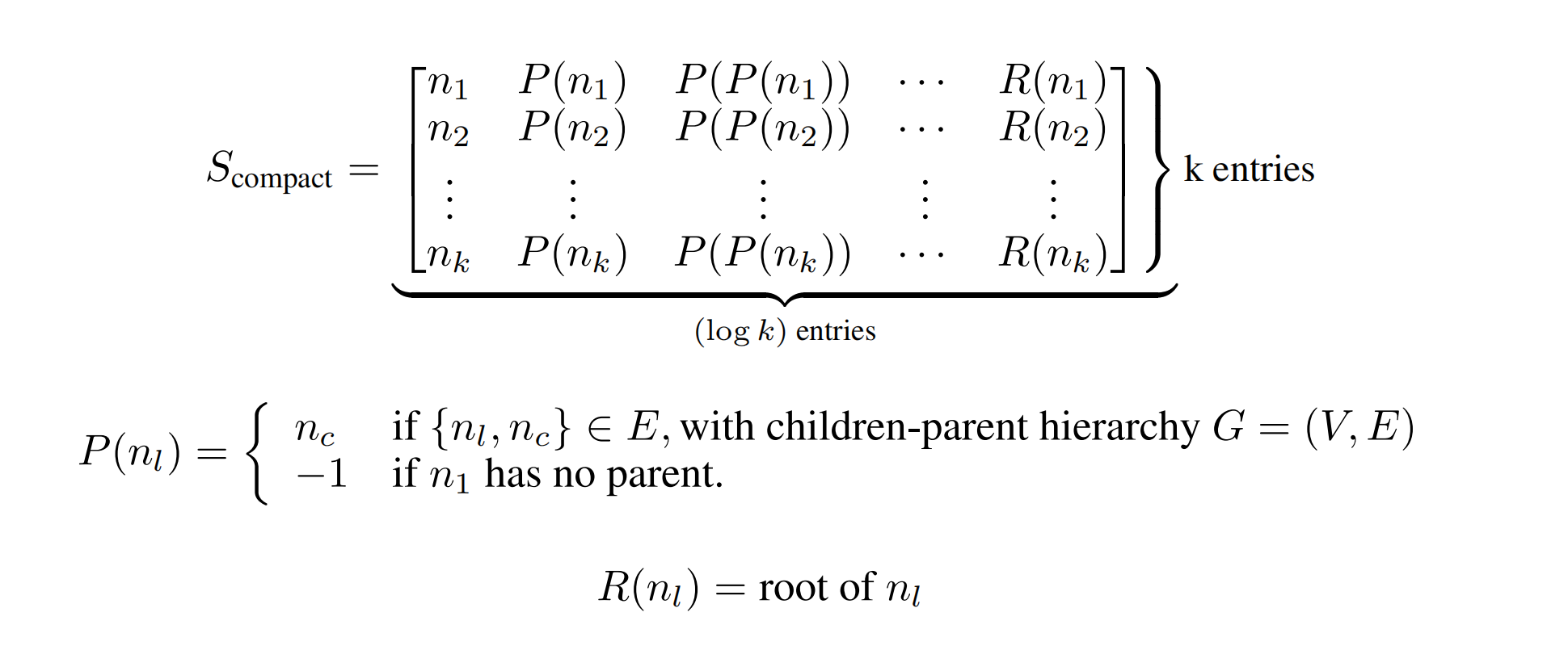
S_compact utilizes the fact that all contributions of a node in the hierarchy in the summing matrix is it's path to root. It is also important to note that S_compact is storage efficient and workload mapping-friendly: all non- − 1 entries of S_compact are exactly the non-zero entries in S, and a parallel machine can easily map rows of S_compact to primitives to achieve speedup in summation matrix construction (OpenMP threads in our implementation, or alternatively SIMD gangs or CUDA threads).

The second remark is that little constraints are placed on the order of nodes in existing implementations, which means that many sequences of reconciliation by G and summation by S exists. We instead impose "Constrained Ordering", which enforces that all leaf nodes have ID between 0 and k, and all non-leaf nodes occupy the rest of the IDs. Not only does this make construction of G and S easily parallelizable and maintainable, but also paves the way for algorithmic optimizations (e.g. reconciliation of a leaf forecast in a bottom-up case is the identity transformation explained below.

Large-scale Hierarchical Time-series Reconciliation Benchmark

To perform accurate stress-tests of forecast reconciliation algorithms require novel, large-scale benchmarks. To this end, we present three newly designed benchmarks (M5-Full, M5-Hobbies, Wikipedia) that are orders-of-magnitude larger than their counterparts in existing academic literature. Figure [fig:bench] provides a description and compares key characteristics of the proposed benchmarks. All data comes with the hierarchy in compact storage format, historicals, and forecasts using Prophet [Taylor and Letham] for the last 100 time-stamps available.

Dataset	Source	# Leaves	# Nodes	# Levels
TourismSmall	[Izenman, 2013]	56	89	4
Labour	[Olivares et al., 2022]	32	57	4
M5-Hobbies	All "Hobbies" sales data from [Kaggle, a]	5650	6218	4
M5-Full	All sales data from [Kaggle, a]	30490	33549	4
Wikipedia	All visits data from [Kaggle, b]	145063	308004	4

Implementation Details and Problem Mapping

The LHTS (large-scale hierarchical time-series reconciliation) package is a Python library that enables data scientists to easily access a parallel system for reconciling large hierarchical time-series datasets in single CPU-node, multi-process, and multi CPU-node settings. The core component is implemented in C++ with OpenMPI, OpenMP, and Eigen (a popular LAPACK/BLAS replacement), and is connected to Python via pybind11. It is built using setuptools and CMake, allowing users to easily call highly-optimized routines that leverage SIMD, threaded-parallelism, and message-passing with NumPy arrays produced in the same Python process. This is often useful for existing forecasts produced by frameworks like PyTorch, sklearn, Prophet, or Nixtla.

The package provides implementations of naive single-process and MPI solutions for five popular reconciliation algorithms (bottom-up, top-down, middle-out OLS, WLS) in both sparse and dense versions, as well as two techniques leveraging data parallelism similar to those used in deep learning. Benchmarks indicate that the single-process C++ implementation is 25x faster than Nixtla in top-down and middle-out methods, and the data-parallel communication reduction technique is 25% faster than its naive MPI counterpart. The results of our experiments also demonstrate the trade-offs of different methods offered by LHTS.

During development, we drew inspiration from implementations in Nixtla as well as sample CMake projects using pybind11. Forecasts are mapped to the processes they originate from, and matrix multiplication between S and G is marked for either SIMD execution or sequential execution based on the matrix type (dense vs sparse). Multiplication between ŷ and SG is marked for SIMD execution. Construction of S and G is marked for threaded OpenMP execution for increased speed, as presented in the compact storage format. We benchmarked our solutions using two Google Cloud Platform e2-highcpu-16 instances with 1 vCPU per core, 8 cores, and an Intel Broadwell x86/64 architecture, one located in us-central1-a and the other in us-east1-b1.

Single-Process Optimizations

The traditional forecast reconciliation algorithm, such as Nixtla, is a single-process solution that relies on dense matrix operations, which can be a computationally expensive and resource-intensive task, especially when dealing with large matrices. In an effort to improve the performance of this approach, we explored two strategies.

First, we utilized sparse matrices, which require less memory to store and can be processed more efficiently than dense matrices. Specifically, we used Eigen's [Guennebaud et al., 2010] sparse matrix operations to multiply the sparse matrices S and G (which represent the hierarchy and flow of forecasts, respectively) with the dense matrix ŷ, representing incoherent forecast predictions. Our implementation of this strategy resulted in significant performance improvements.

Alternatively, we reconstructed the matrix operations using algorithms that perform the same tasks and implemented OpenMP to execute them in parallel using multiple threads. While this approach did improve the performance of the dense matrix solution, the improvement was not as significant as the sparse matrix approach. Here are some core insights to algorithmic optimization opportunities in each reconciliation algorithm where this is possible:

• Bottom-up: Instead of reconciling through G, all forecasts after num_leaves rows could be thrown out, and we should only apply summation by S.

• Top-down: Instead of reconciling through G, distribute the forecasts from root to each leaf in parallel using OpenMP, then sum up by S.

• Middle-out: Instead of reconciling through G, distribute the forecasts from the given level to each leaf in parallel using OpenMP, then sum up by S.

To fully optimize the performance of the forecast reconciliation algorithm, we propose a hybrid approach that combines the use of sparse-sparse matrix multiplication between S and G (which is inherently sequential, but much faster than the SIMD dense-dense alternative) with SIMD techniques for the sparse-dense matrix multiplication between SG and ŷ. This combination leverages the strengths of both approaches to deliver the most efficient solution.

Multiple-Process Optimizations

To implement our multiple-process algorithm, we utilized message-passsing primitives in OpenMPI. As the forecasting algorithm Prophet can be run in parallel using either OpenMP or MPI, our hierarchy and forecast values could be distributed across multiple processes before reconciliation. The task executed by each process is then defined as producing the correct reconciliation of the locally produced forecast taking into consideration all forecasts and the entire hierarchy, not just local hierarchy. For the sake of simplicity (and making note that hierarchy remains unchanged), each process will have the entire hierarchy available in-memory at the beginning of the reconciliation process, in compact storage format.

We present two classes of approach: gather-based and data-parallelism (dp) based. We also provide an alternative version of the data-parallelism that provides speed-up in certain scenarios.

In the gathered-based approach, all processes send forecasts to a single process that performs the reconciliation before distributing the results back to each process. This results in fewer messages being communicated throughout the network, but a larger amount of information being transmitted. Additionally, the process performing the reconciliation may not have access to all available resources and is confined to the physical cores available in a shared memory region. In a multi-node configuration, this means that the computation is restricted to a single node.

An alternative strategy was to implement data parallelism. In this model, each process obtained a slice of SG that was relevant to its own forecast and performed reconciliation at the same time. The optimized variant was inspired by single-process algorithmic optimization techniques and aimed to reduce communication through the nature of each type of reconciliation algorithm. Only processes that are determined to have to communicate (e.g. between leaves and root in bottom-up, and between root and leaves in top-down) will communicate their chunks of forecasts in a point-to-point fashion. This reduced the total amount of information transmitted, but increased the number of messages being sent. Additionally, since each process now performs heavy computation, fine-grained interactions between the forecast hierarchy, OpenMPI processes, shared memory regions, and OpenMP threads can lead to redundant computation (in obtaining and slicing SG) and context switching costs.

Results

Single-Process Performance Results

On Dataset M5-Hobbies

Time Performance: We observed a significant improvement in time performance when applying OpenMP to optimize our dense-matrix implementation for the M5-Hobbies dataset, resulting in a 50x speedup. Utilizing a sparse matrix also led to a significant increase in performance, with a speedup of over 500x compared to the dense-matrix solution. However, the application of OpenMP on the sparse-matrix solution did not provide any additional improvement. This may be because the sparse-matrix solution already requires a larger portion of the matrices and more computation, and the overhead of parallelization cannot be offset by the already efficient nature of the sparse-matrix solution.

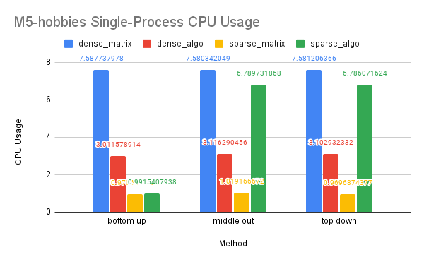
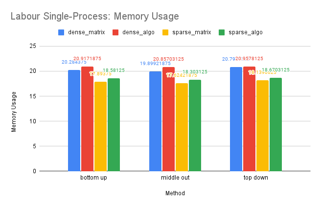
CPU and Memory Usage: Our analysis of CPU usage revealed that the OpenMP dense-algo solution significantly reduced CPU usage in the dense-matrix implementation. This may be due to the algorithm solution requiring less computation than the purely matrix solution, as well as OpenMP’s ability to divide the work among multiple threads that can be executed in parallel on different processors or cores. The sparse-matrix solution demonstrated the lowest CPU usage, likely because sparse matrices and their computations are inherently sequential in Eigen. However, the sparse-algo solution showed a higher CPU usage, which may be attributed to the solution storing and computing a larger portion of the matrices than the purely matrix solution and the frequent contention of multiple threads accessing shared variables.

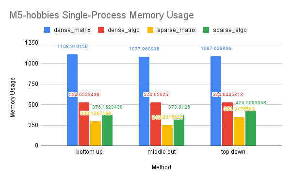
Our analysis of memory usage showed that the dense-algo solution had lower memory usage than the dense-matrix solution. This may be due to the algorithm solution allocating less space for the matrices and requiring less matrix computation than the purely matrix solution. The sparse-matrix solution had the lowest memory usage, as sparse matrices require less memory to store than dense matrices. However, the sparse-algo solution allocated more memory space to access a larger portion of the matrices, which may result in higher memory usage compared to the sparse-matrix solution.

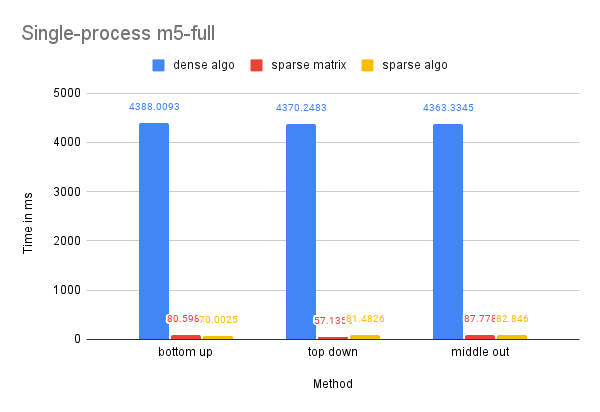
On Dataset M5-Full

Time Performance: As this dataset is larger than the previous one, the dense-matrix solution experienced a memory outage. The utilization of sparse matrices addressed this problem and resulted in a significant speedup of over 50 times. While OpenMP did not have a notable effect on the efficiency of the sparse-matrix-based solution, this could be due to the already optimized nature of the solution and the inability to conceal the overhead of parallelization with improvements.

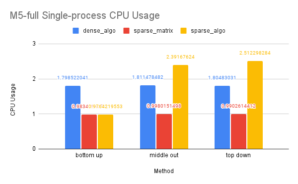
CPU and Memory Usage: The trend in CPU and memory usage for this dataset is comparable to that of the M5-Hobbies dataset, likely due to similar underlying causes.

On Dataset Wikipedia

Time Performance: As this is the largest dataset we have tested, the dense solution encountered an our-of-memory error. The sparse-algo solution using OpenMP was slower than the sparse-matrix solution, possibly because the sparse-matrix solution was already efficient and the overhead of parallelization could not be concealed by improvements.

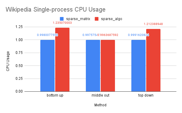
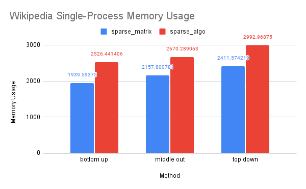
CPU and Memory Usage: The trend in CPU and memory usage for this dataset mirrors that of the previous two datasets, likely due to similar underlying causes. However, we noticed that the differences in CPU and memory usage between the sparse-algo and sparse-matrix solution were less pronounced compared to the previous two datasets. This may be due to the fact that the Wikipedia dataset is large enough that the differences between the matrices accessed and computed by the two solutions narrowed.

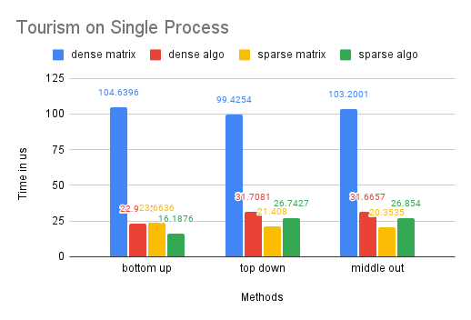
On Dataset Tourism

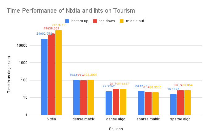
Time Performance: We can observe that the performance of our optimized dense-matrix solution using OpenMP and our sparse-matrix solution improved by about 3 times compared to the traditional dense-matrix solution. However, the improvement between the dense-algo and sparse-matrix and sparse-algo is limited. This is likely due to the smaller size of this dataset compared to the previous ones.

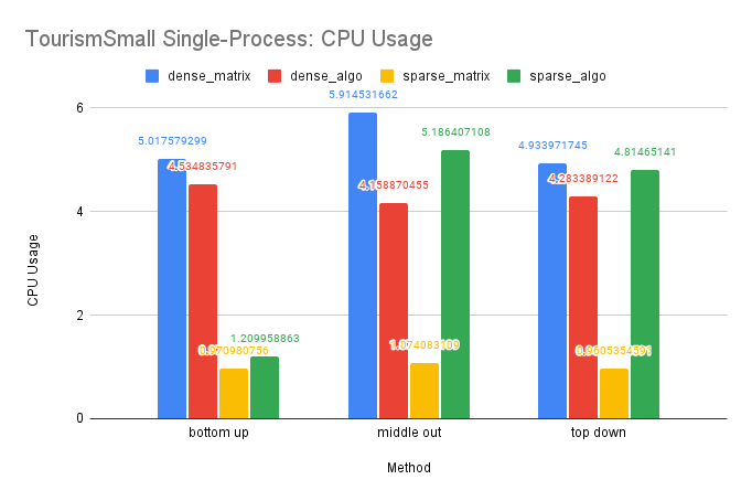
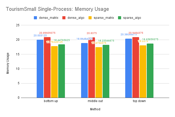
CPU and Memory Usage: The trend in CPU usage for this dataset is similar to that of the M5-Hobbies dataset, likely due to similar underlying causes. However, the improvement in CPU usage by OpenMP is less pronounced on this smaller dataset. Additionally, the small size of the dataset may cause the sparse matrices to resemble dense matrices in memory storage, resulting in similar memory usage for the sparse and dense solutions, as well as similar memory usage between the sparse-algo and sparse-matrix solutions.

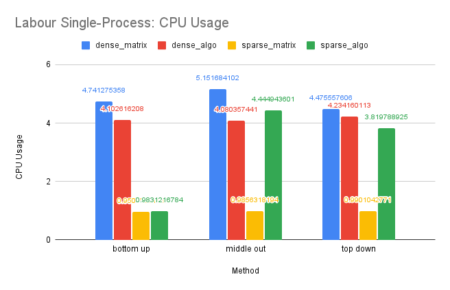
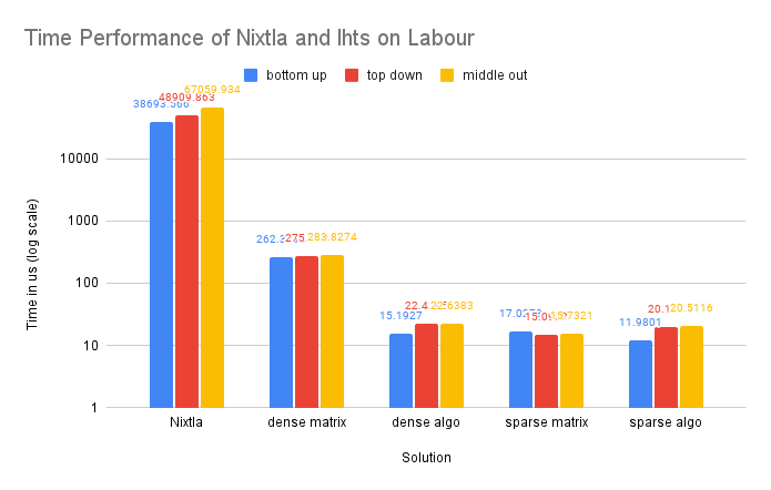
On Dataset Labour

Time Performance: The trend in time performance for this dataset is similar to that of the Tourism dataset, likely due to similar underlying causes.

CPU and Memory Usage: The CPU and memory usage of this dataset shows similar trend as the Tourism dataset for similar reasons.

Multiple-Process Performance Results

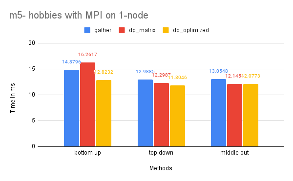
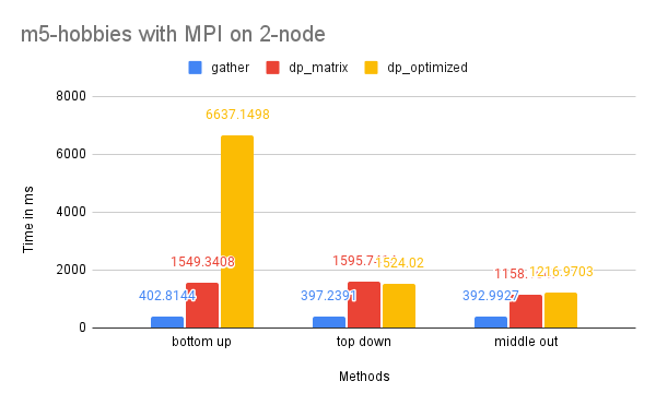
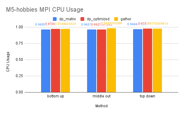
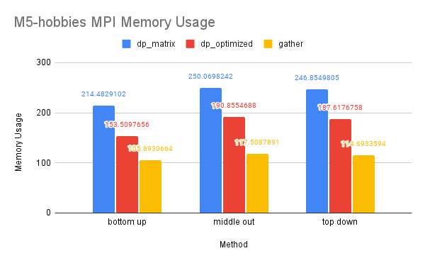
On Dataset M5-Hobbies

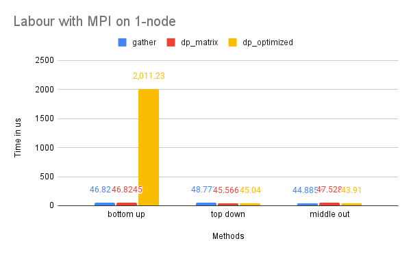
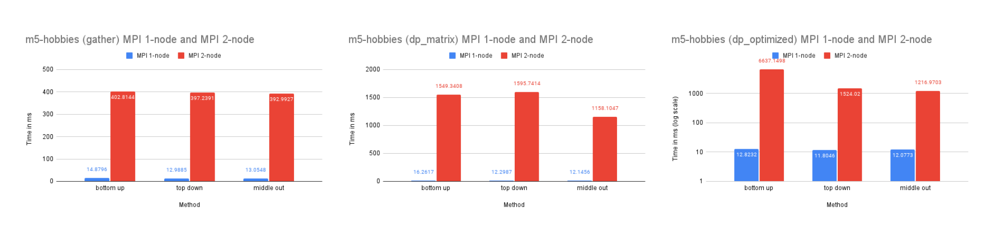
Time Performance: As the graph illustrates, the dp-optimized solution performs slightly better than dp-matrix and the naive gather solutions on one node.

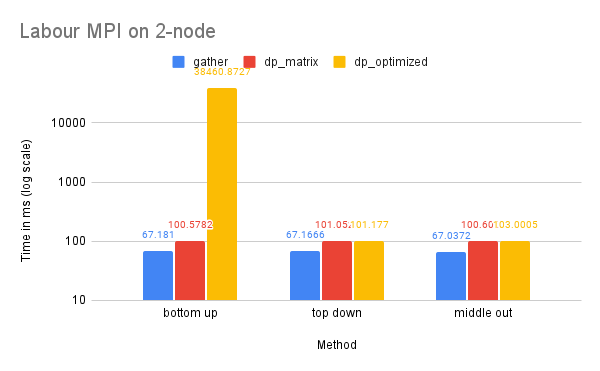
On two nodes, gather performs better in terms of time due to its simpler communication pattern. Additionally, the bottom-up dp-optimized method is much slower than the other solutions because the data (the leaves) are highly interdependent during the computation process and require more scattered communication.

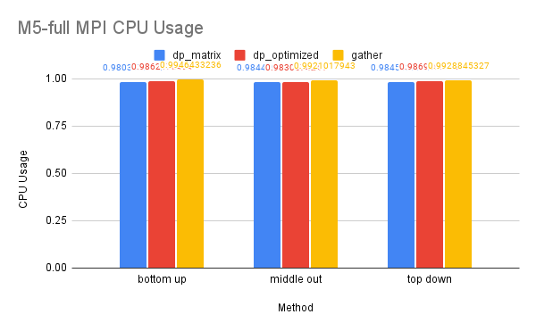
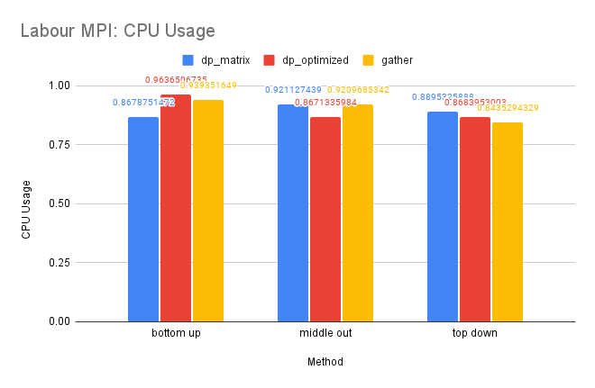
CPU and Memory Usage: The CPU usage of the three methods is similar because they require a similar amount of computation in total. The gather method uses the least amount of memory, while the dp-matrix method uses the most. This is because gather has few data dependencies and requires less memory storage for shared variables in MPI.

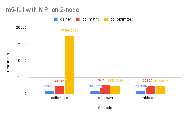
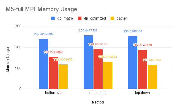
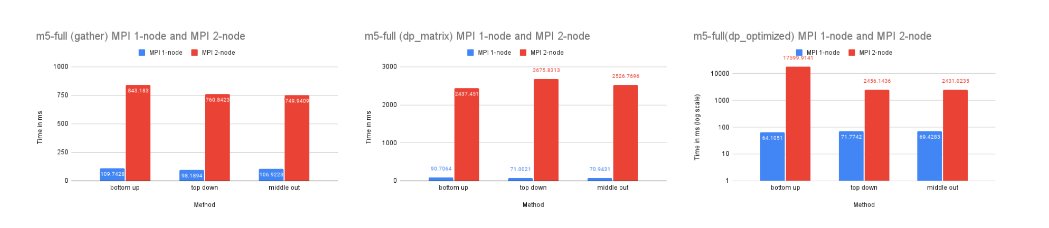
On Dataset M5-Full

Time Performance: As the graph shows, the dp-matrix and dp-optimized solutions perform better than dp-matrix and the naive gather solutions on one node due to the larger size of the dataset, which benefits more significantly from parallelized computation.

The time performance on two nodes is similar to that of the M5-Hobbies dataset for similar reasons.

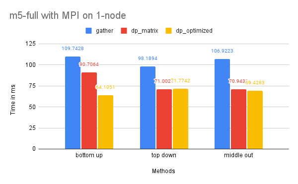
CPU and Memory Usage: The CPU and memory usage of this dataset resembles the trend of the previous dataset for similar reasons.

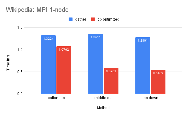
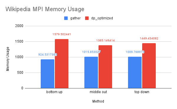
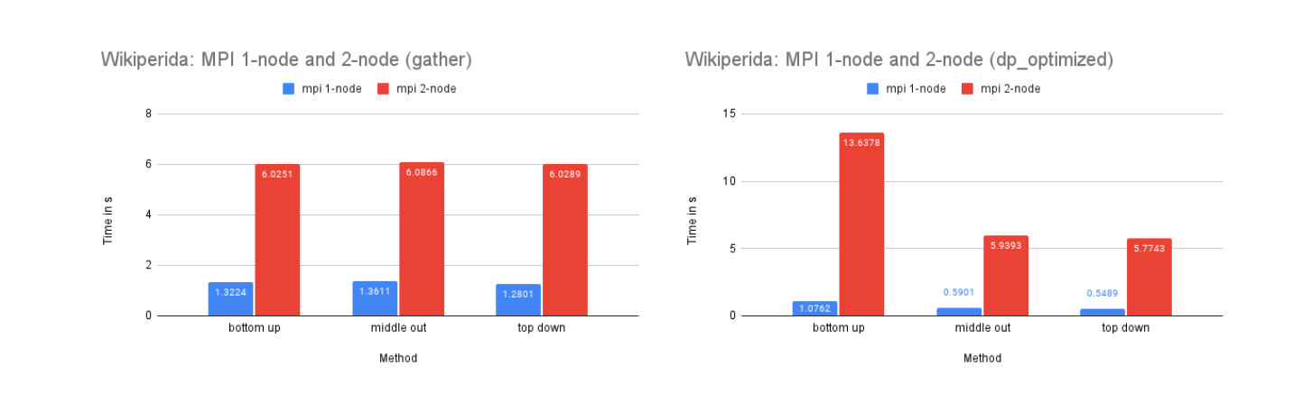
On Dataset Wikipedia

Time Performance: The dp-matrix solution encountered an out-of-memory error. The time performance on one node of this dataset is similar to that of the M5-full dataset for similar reasons.

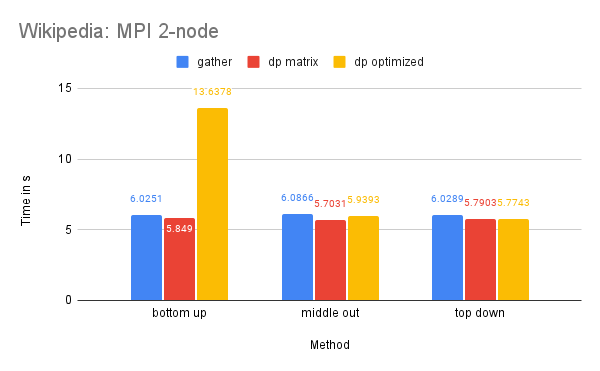
On two nodes, we have sufficient memory for the dp-matrix solution due to the additional memory availability. The Wikipedia dataset is larger, which means that the benefits of parallelized computation are greater, making the scattered communication cost of dp-matrix and dp-optimized less impactful.

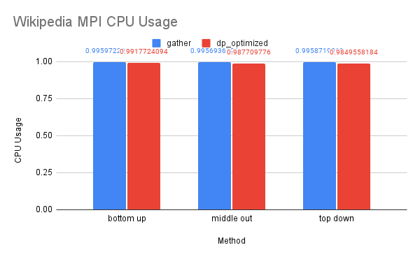
CPU and Memory Usage: The dp-matrix solution was out of memory on 1-node. The CPU and memory usage of this dataset resembles the trend of the previous dataset for similar reasons.

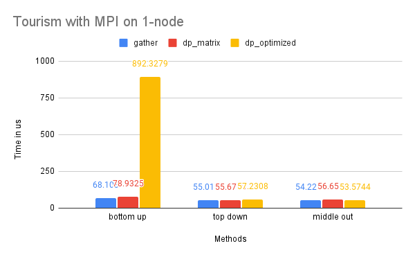
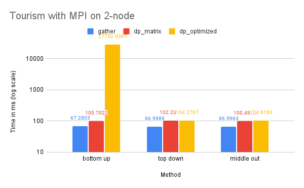
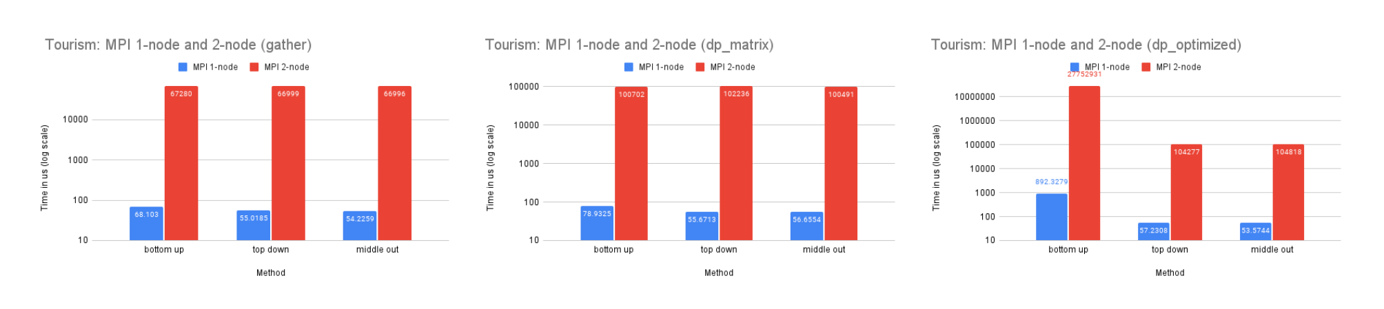
On Dataset Tourism

Time Performance: The smaller size of this dataset renders the benefits of utilizing multiple processes for computation minimal, and the high communication cost of the dp-optimized solution significantly diminishes its time performance. This is also reflected in the time performance of Tourism on 2-node, which is similar to that of M5-hobbies for similar reasons.

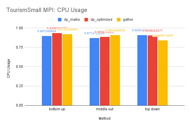
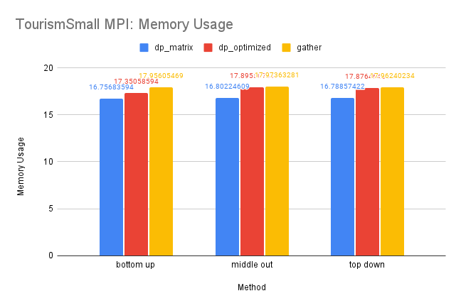
CPU and Memory Usage: The CPU usage of the three methods are similar for reasons discussed above. And since this dataset is small, the differences between the memory usage is also insignificant since there is less information needed for storage.

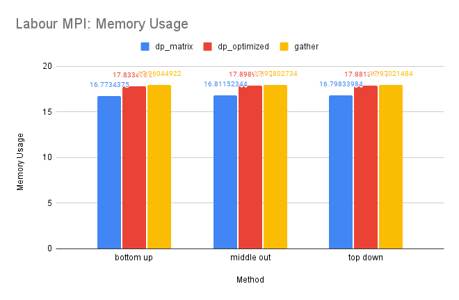
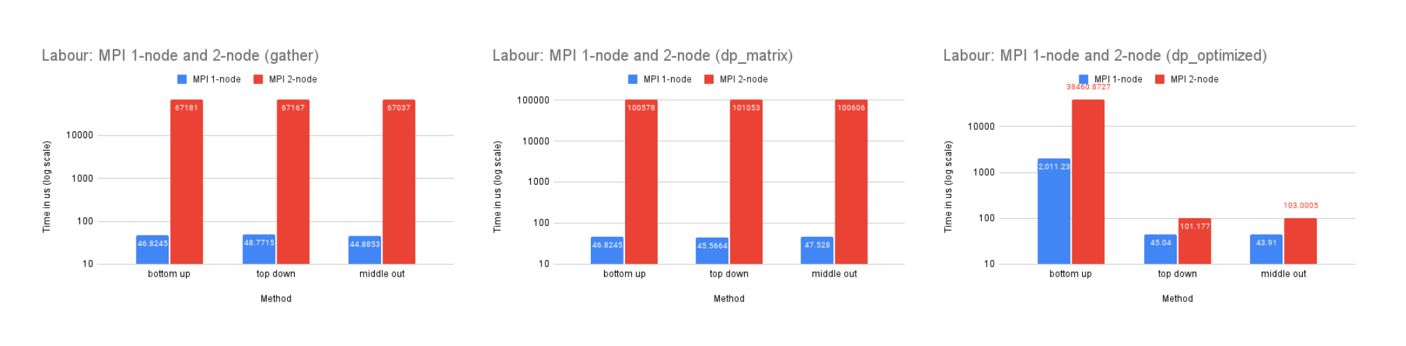
On Dataset Labour

Time Performance: The time performance of this dataset resembles the trend of the Tourism dataset for similar reasons.

CPU and Memory Usage: The CPU and memory usage of this dataset resembles the trend of the Tourism dataset for similar reasons.

Single-Process Compared with Nixtla

We only tested Nixtla on smaller datasets, as it is not designed for large-scale processing. Our single-process implementation utilizing dense matrices and written in C++ achieved hundreds of times faster performance compared to the Nixtla implementation in Python. Additionally, our sparse implementation exhibited over 2000 times faster performance compared to the Nixtla dense-matrix implementation.

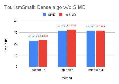
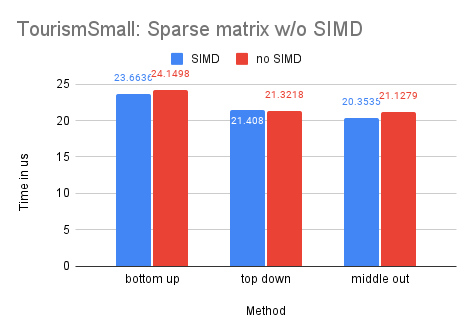
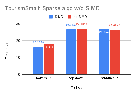
Single-Process with and without SIMD

On Dataset M5-hobbies

Our results demonstrate that the dense-matrix solution experienced the greatest improvement from SIMD, with a speedup of approximately 7x. The dense-algo solution also benefited from SIMD, performing about 1.4x faster than without it. However, this improvement was less significant compared to the dense-matrix solution, potentially due to the smaller amount of computation required for the dense-algo solution and the overhead introduced by OpenMP parallelization. The impact of SIMD on the sparse-matrix solution was relatively limited, and it even had a negative effect on the sparse-algo solution due to the smaller size of the computation and the overhead of parallelization.

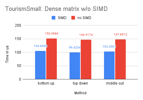
On Dataset Tourism

As the Tourism dataset is smaller in size compared to the M5-Hobbies dataset, the potential benefits of utilizing SIMD technology are significantly reduced. In fact, only the dense-matrix solution demonstrates a notable improvement in performance, with a speedup of approximately 1.4 times. The other solutions show little to no improvement upon implementing SIMD.

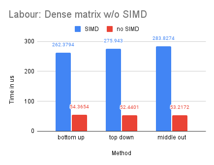
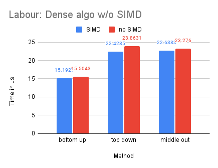
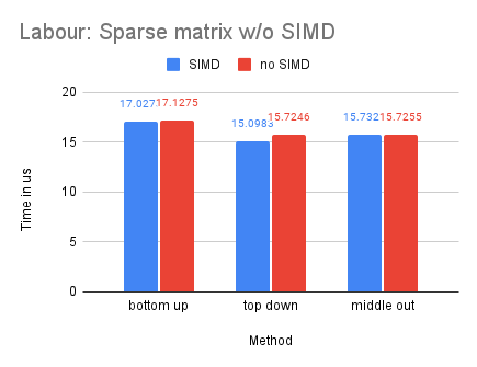
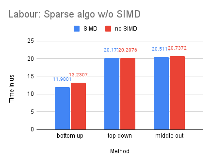
On Dataset Labour

With Labour being our smallest dataset, we observe that the dense-matrix solution is slower with SIMD, potentially due to the high overhead of parallelization.

Multiple-Process (MPI) Compared with Single Process

Our implementation of the MPI multiple-process approach did not yield significant speed improvements compared to the optimized single-process implementations, with the exception of the Wikipedia dataset, which showed a speedup of approximately 2 times. This lack of improvement can be interpreted as a difference in settings - in a single-process scenario, all forecasts are situiated in the same process in continugous memory already, which is not the case for the MPI scenario. There is also little difference in CPU usage between the single-process solution and the MPI solution for similar reasons.

Multiple-Process on 1-Node and 2-Node

Our analysis reveals that the MPI implementation performs significantly slower on a two-node system compared to a single-node system for all datasets, although the magnitude of this difference decreases as the dataset size increases. This is likely due to the high network latency between the two nodes, as well as the communication complexity involved in distributing the workload. However, as the size of the dataset increases, the benefits of utilizing the additional resources and memory storage provided by the two-node system become more significant, leading to a decrease in the performance gap between the single-node and two-node configurations.

Integration with Data Science Workload

In our artifacts, we hae also demonstrated a simple integration of LHTS into a data science workload. The user could launch a multi-process Python script to train a forecasting model on a large dataset over many processes, and readily reconcile them using our LHTS by calling functions distrib.reconcile_dp_optimized with distrib = lhts.Distributed(), and calculate performance metrics using functions like lhts.smape(yhat, gt).

Conclusion

The manuscript proposes the design and implementation of LHTS to perform large-scale forecast reconciliation with the following components,

• A dense-matrix based single-process solution (dense-matrix)

• A dense-matrix based single-process solution with OpenMP (dense-algo)

• A sparse-matrix based single-process solution (sparse-matrix)

• A sparse-matrix based single-process solution with OpenMP (sparse-algo)

• A naive MPI solution that only parallelized the loading of matrices (gather)

• An MPI solution that utilizes data-parallelism (dp-matrix)

• An MPI solution that utilizes data-parallelism with optimized communication (dp-optimized)

We tested these solutions on Google Cloud Platform VM instances using the Labour, Tourism, M5-hobbies, M5-full, and Wikipedia datasets (ranked from smallest to largest).

Overall, our dense-matrix single-process implementation with SIMD achieved hundreds of times speedup on smaller datasets such as Tourism and Labour, and a further 50x+ speedup with OpenMP parallelization on larger datasets like M5-Hobbies. Our sparse-matrix single-process implementation also provided significant improvements in time performance and CPU and memory usage on larger datasets.

Our multi-process implementation with MPI achieved significant improvements in time performance or CPU usage on our largest dataset, Wikipedia. In single-node experiments, data parallelism-based solutions performed better, while gather-based methods performed better in multi-node experiments due to lower number of message sent. However, the slow link present in multi-node experiments exacerbated the communication problem, highlighting the need for communication-aware and computation-optimized large-scale hierarchical time-series forecast reconciliation algorithms like LHTS.

References

George Athanasopoulos, Rob J. Hyndman, Nikolaos Kourentzes, and Fotios Petropoulos. Forecasting with temporal hierarchies. European Journal of Operational Research, 262(1):60–74, 2017. ISSN 0377-2217. doi: https://doi.org/10.1016/j.ejor.2017.02.046. URL https://www.sciencedirect.com/science/article/pii/S0377221717301911.

Gaël Guennebaud, Benoît Jacob, et al. Eigen v3. http://eigen.tuxfamily.org, 2010.

Rob Hyndman and G. Athanasopoulos. Forecasting: Principles and Practice. OTexts, Australia, 3rd edition, 2021.

Rob J. Hyndman, Roman A. Ahmed, George Athanasopoulos, and Han Lin Shang. Optimal combination forecasts for hierarchical time series. Computational Statistics & Data Analysis, 55(9):2579–2589, 2011. ISSN 0167-9473. doi: https://doi.org/10.1016/j.csda.2011.03.006. URL https://www.sciencedirect.com/science/article/pii/S0167947311000971.

Alan Julian Izenman. Modern multivariate statistical techniques. In Springer Texts in Statistics, Springer texts in statistics, pages 315–368. Springer New York, New York, NY, 2013.

Kaggle. M5 forecasting - accuracy, a. URL https://www.kaggle.com/competitions/m5-forecasting-accuracy/overview/evaluation.

Kaggle. Web traffic time series forecasting, b. URL https://www.kaggle.com/competitions/web-traffic-time-series-forecasting.

C. L. Lawson, R. J. Hanson, D. R. Kincaid, and F. T. Krogh. Basic linear algebra subprograms for fortran usage. ACM Trans. Math. Softw., 5(3):308–323, sep 1979. ISSN 0098-3500. doi: 10.1145/355841.355847. URL https://doi.org/10.1145/355841.355847.

Kin G. Olivares, Federico Garza, David Luo, Cristian Challú, Max Mergenthaler, and Artur Dubrawski. Hierarchicalforecast: A reference framework for hierarchical forecasting in python. Computing Research Repository, abs/2207.03517, 2022. URL https://arxiv.org/abs/2207.03517.

Anastasios Panagiotelis, George Athanasopoulos, Puwasala Gamakumara, and Rob J. Hyndman. Forecast reconciliation: A geometric view with new insights on bias correction. International Journal of Forecasting, 37(1):343–359, 2021. ISSN 0169-2070. doi: https://doi.org/10.1016/j.ijforecast.2020.06.004. URL https://www.sciencedirect.com/science/article/pii/S0169207020300911.

Sean J Taylor and Benjamin Letham. Forecasting at scale — peerj.com. https://peerj.com/preprints/3190/. [Accessed 16-Dec-2022].

Shanika L. Wickramasuriya, George Athanasopoulos, and Rob J. Hyndman. Optimal forecast reconciliation for hierarchical and grouped time series through trace minimization. Journal of the American Statistical Association, 114(526):804–819, 2019. doi: 10.1080/01621459.2018.1448825. URL https://doi.org/10.1080/01621459.2018.1448825.